物种分布建模示例简介

代码实现[Python]

# -*- coding: utf-8 -*-  # Authors: Peter Prettenhofer  #          Jake Vanderplas  # # License: BSD 3 clause from time import time import numpy as np import matplotlib.pyplot as plt from sklearn.datasets.base import Bunch from sklearn.datasets import fetch_species_distributions from sklearn.datasets.species_distributions import construct_grids from sklearn import svm, metrics # 如果basemap可用，则使用basemap绘制边界；否则自行处理实现。 try: from mpl_toolkits.basemap import Basemap
    basemap = True except ImportError:
    basemap = False print(__doc__) # 创建物种种群：基于物种名从训练集和测试集提取信息 def create_species_bunch(species_name, train, test, coverages, xgrid, ygrid): """Create a bunch with information about a particular organism

    This will use the test/train record arrays to extract the
    data specific to the given species name.
    """ bunch = Bunch(name=' '.join(species_name.split("_")[:2]))
    species_name = species_name.encode('ascii')
    points = dict(test=test, train=train) for label, pts in points.items(): # choose points associated with the desired species pts = pts[pts['species'] == species_name]
        bunch['pts_%s' % label] = pts # determine coverage values for each of the training & testing points ix = np.searchsorted(xgrid, pts['dd long'])
        iy = np.searchsorted(ygrid, pts['dd lat'])
        bunch['cov_%s' % label] = coverages[:, -iy, ix].T return bunch # 绘制种群分布 def plot_species_distribution(species=("bradypus_variegatus_0", "microryzomys_minutus_0")): """
    Plot the species distribution.
    """ if len(species) > 2:
        print("Note: when more than two species are provided," " only the first two will be used")

    t0 = time() # Load the compressed data data = fetch_species_distributions() # Set up the data grid xgrid, ygrid = construct_grids(data) # The grid in x,y coordinates X, Y = np.meshgrid(xgrid, ygrid[::-1]) # create a bunch for each species BV_bunch = create_species_bunch(species[0],
                                    data.train, data.test,
                                    data.coverages, xgrid, ygrid)
    MM_bunch = create_species_bunch(species[1],
                                    data.train, data.test,
                                    data.coverages, xgrid, ygrid) # background points (grid coordinates) for evaluation np.random.seed(13)
    background_points = np.c_[np.random.randint(low=0, high=data.Ny,
                                                size=10000),
                              np.random.randint(low=0, high=data.Nx,
                                                size=10000)].T # We'll make use of the fact that coverages[6] has measurements at all # land points.  This will help us decide between land and water. land_reference = data.coverages[6] # Fit, predict, and plot for each species. for i, species in enumerate([BV_bunch, MM_bunch]):
        print("_" * 80)
        print("Modeling distribution of species '%s'" % species.name) # Standardize features mean = species.cov_train.mean(axis=0)
        std = species.cov_train.std(axis=0)
        train_cover_std = (species.cov_train - mean) / std # Fit OneClassSVM print(" - fit OneClassSVM ... ", end='')
        clf = svm.OneClassSVM(nu=0.1, kernel="rbf", gamma=0.5)
        clf.fit(train_cover_std)
        print("done.") # Plot map of South America plt.subplot(1, 2, i + 1) if basemap:
            print(" - plot coastlines using basemap")
            m = Basemap(projection='cyl', llcrnrlat=Y.min(),
                        urcrnrlat=Y.max(), llcrnrlon=X.min(),
                        urcrnrlon=X.max(), resolution='c')
            m.drawcoastlines()
            m.drawcountries() else:
            print(" - plot coastlines from coverage")
            plt.contour(X, Y, land_reference,
                        levels=[-9998], colors="k",
                        linestyles="solid")
            plt.xticks([])
            plt.yticks([])

        print(" - predict species distribution") # Predict species distribution using the training data Z = np.ones((data.Ny, data.Nx), dtype=np.float64) # We'll predict only for the land points. idx = np.where(land_reference > -9999)
        coverages_land = data.coverages[:, idx[0], idx[1]].T

        pred = clf.decision_function((coverages_land - mean) / std)
        Z *= pred.min()
        Z[idx[0], idx[1]] = pred

        levels = np.linspace(Z.min(), Z.max(), 25)
        Z[land_reference == -9999] = -9999 # plot contours of the prediction plt.contourf(X, Y, Z, levels=levels, cmap=plt.cm.Reds)
        plt.colorbar(format='%.2f') # scatter training/testing points plt.scatter(species.pts_train['dd long'], species.pts_train['dd lat'],
                    s=2 ** 2, c='black',
                    marker='^', label='train')
        plt.scatter(species.pts_test['dd long'], species.pts_test['dd lat'],
                    s=2 ** 2, c='black',
                    marker='x', label='test')
        plt.legend()
        plt.title(species.name)
        plt.axis('equal') # Compute AUC with regards to background points pred_background = Z[background_points[0], background_points[1]]
        pred_test = clf.decision_function((species.cov_test - mean) / std)
        scores = np.r_[pred_test, pred_background]
        y = np.r_[np.ones(pred_test.shape), np.zeros(pred_background.shape)]
        fpr, tpr, thresholds = metrics.roc_curve(y, scores)
        roc_auc = metrics.auc(fpr, tpr)
        plt.text(-35, -70, "AUC: %.3f" % roc_auc, ha="right")
        print("\n Area under the ROC curve : %f" % roc_auc)

    print("\ntime elapsed: %.2fs" % (time() - t0))


plot_species_distribution()
plt.show()

代码执行

代码运行时间大约:0分20.185秒。
运行代码输出的文本内容如下，分别给出了2个物种的OneClassSVM建模AUC结果。

________________________________________________________________________________
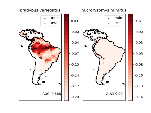
Modeling distribution of species 'bradypus variegatus'
 - fit OneClassSVM ... done.
 - plot coastlines from coverage
 - predict species distribution

 Area under the ROC curve : 0.868443
________________________________________________________________________________
Modeling distribution of species 'microryzomys minutus'
 - fit OneClassSVM ... done.
 - plot coastlines from coverage
 - predict species distribution

 Area under the ROC curve : 0.993919

time elapsed: 20.18s

运行代码输出的图片内容如下，图中2个物种的分布密度情况一目了然。

源码下载

• Python版源码文件: plot_species_distribution_modeling.py
• Jupyter Notebook版源码文件: plot_species_distribution_modeling.ipynb